Hardware Profiling - The math behind the idea

Overview

The system uses a Wiener H1 estimator accumulated across multiple sine sweep passes, where each frequency bin's transfer function H[k] is regularized by a frequency-dependent term λ_k that automatically suppresses noisy high-frequency bins — the log sweep's naturally falling energy density leaves reference power low at high frequencies, and the regularizer grows to compensate. A smoothing window capping mechanism limits the 1/3-octave averaging window so that above-cutoff zero bins are excluded, eliminating the artificial peak artifact that would otherwise appear near the Nyquist boundary. System loopback calibration captures the audio interface and cable coloration as a separate estimate H_sys[k] and divides it out of every subsequent device measurement, so the fitted filter and waveshaper tables reflect only the device under test and not the measurement rig. Together — frequency-dependent regularization, smoothing boundary capping, and loopback calibration — these three mechanisms ensure the model is both numerically stable across the full audio band and free of systematic interface coloration.

The system measures the device's nonlinear input-to-output transfer curve at each gain stage, then at playback time interpolates between whichever two neighboring curves bracket the current signal level — letting the saturation character shift dynamically as the signal gets louder or quieter, the way real hardware does.

Screenshots on this post are taken from my complete write-up.

The measurement system is implement as a JUCE standalone desktop application targeting macOS. It provide a real-time audio enginer, a structured capture workflow, and an offline analysis engine that fits the L-N-L model. This model can then be interpreted for accurate plugin recreation of the device.

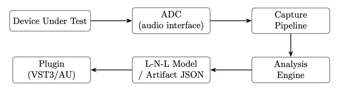
The amount of distortion added by an analog unit is different from setting to setting, so we must design an adaptive process to measure what those spectral differences are to recreate them. The adaptive filter model is a gray-box approach, it fixes the model topology from physical knowledge of analog circuits while estimating parameters from data.

For this project, I use a second-order Volterra kernel to capture the nonlinear memory effects that the memoryless table alone cannot model.

The device is modeled as a a Linear-Nonlinear-Linear cascade where h1 and h2 are the FIR impulse responses and N is a static point-wise nonlinearity.

Frequency-Response Estimation via Wiener Filter

For each SineSweep capture pair (x,y), both signals are zero-padded to the next power-of-two length M and their DFTs are computed. The complex cross-spectrum and reference power spectrum are accumulated over P sweeps:

The Wiener magnitude estimate is

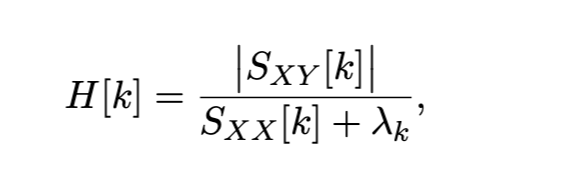
where lambda_k is a frequency-dependent tikhonov regularizer.

Waveshaper Table Fitting

For each sine-tone capture, a 65536-point Hann-windowed FFT is taken of the central region of the recording (avoiding onset and release transients). The fundamental bin k0 is located by peak-finding within ±10 bins of the nominal frequency. THD is computed across harmonics 2–9:

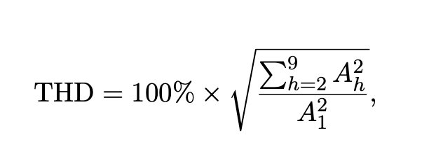
A_h is the peak magnitude near harmonic h. THD is reported per gain label to characterize the onset and degree of saturation. This process essentially maps our different harmonic distortion levels to the gain stage they were at on the original device, ideally mapping the overall tonal color to match the original device when set to the original settings.

Scatter Accumulation

The waveshaper table has T = 1024 bins, uniformly spanning x E [-1, 1]:

For every sample pair (xref[n], yrec[n]) in the analysis window:

Where y is the DC offset of the recording segment, removed to prevent interface or device offsets from biasing the table.

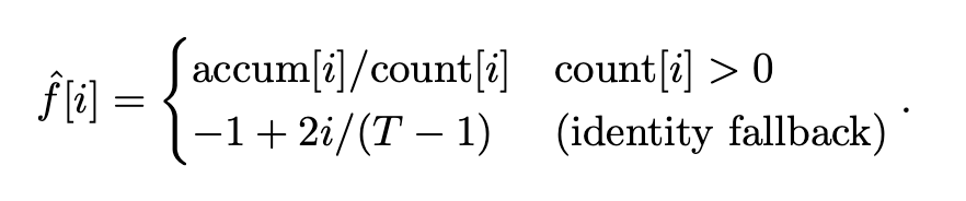
The populated bins are averaged, and gaps are filled by linear interpolation between the nearest populated neighbours. Extreme unpopulated bins are extrapolated using the local slope with an exponential taper to prevent unbounded growth:

L2 Output Filter Identification

Any residual linear coloration after L1 and the waveshaper is identified by running the Wiener estimator on the synthesised L1 ◦ N output versus the actual recording. The L1 convolution is computed via the overlap-add algorithm (block size B = 4096) for O(N log N) complexity.

The models that are derived from the measurement data that you collect with the Analog Hardware Profiler Application are saved as .json files that can be opened in the plugin as a saved model shape.